The coefficients are then further used to derive Wavelet Leaders L(j, k) in the multifractal analysis, as they are the largest coefficients in a certain time neighborhood (local supremum) and possess significant qualities to construct a multifractal formalism (Ref. 16). This can be elaborated by defining dyadic intervals:

(3)

So, the wavelet leaders are defined as:

(4)

Wavelet leaders multifractal formalism (WLMF) in plotting the multifractal spectrum and log cumulants. The structure function derived from the wavelet leaders is defined as:

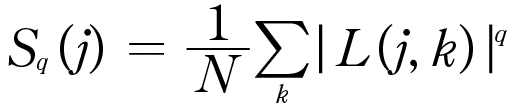
(5)

The scaling function g(q)

(6)

Here, when the cumulant c2=0, the signal is monofractal and has the same scaling in entire data. when c2≠0, the signal is multifractal. The structure function follows a power-law scaling over scales

(7)

The local regularities are described by Hölder exponent h, and the multifractal spectrum D(h) represents the distribution of singularities in the signal.

(8)

Experimentation with Cycloidal Gearbox

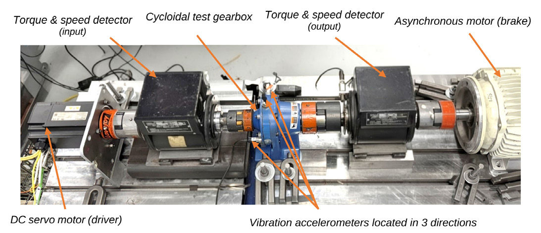
The vibration measurements were carried out on a test stand shown in Figure 3. A Sumitomo cycloidal gearbox of a 15.00:1 ratio was selected for the experiment. CNH-609 gearbox was specifically chosen as it consists of one cycloidal disc (Ref. 17). In lieu of the second disc, which exists in a typical cycloidal reducer, this gearbox design uses a counterweight to achieve dynamic balancing (refer to Figure 1). The one-disc mechanism simplifies the analysis and allows focusing on certain frequencies. In the setup, the gearbox was driven by a DC Servo motor with an encoder feedback loop to provide a consistent speed of 1,800 rpm (30 Hz). The DC motor’s torque capacity was 2.39 Nm. The output shaft of the gearbox was connected to the asynchronous motor that acted as a brake. The torque and speed were measured using torque meters and encoders, respectively, for both input and output shafts. Three vibration sensors (sensitivity 87 mV/g at 6000 CPM) were mounted on the gearbox to collect tri-axial vibration data. All measurements were recorded using the National Instruments Data Acquisition (NI DAQ) system at a sample rate of 12.8 kHz for vibration and 10 kHz for torque measurements. For the input shaft spinning at 30 Hz, the DAQ system would generate 426 and 333 data points for vibration and torque, respectively, in one revolution of the shaft.

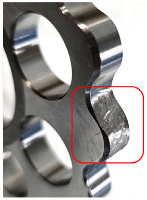
The gearbox was assembled with the standard lubricant using an NGLI 00 grade grease, with a predefined quantity. To confirm that all test iterations were performed at a steady temperature, the test stand was placed in a climate-controlled room with an ambient temperature of 21°C. Two temperature probes were placed to monitor the reduction housing or ‘ring gear’ housing of the gearbox. The load on the reducer output shaft was varied from 0 Nm to 15 Nm during the experimentation. The gearbox was tested for a healthy condition, meaning it had no induced errors. Then it was tested for a worn-out cycloidal disc or damaged condition by swapping out the normal disc with the one seen in Figure 4. Other than the disc, the use of the same parts in both conditions ensured that there were no other changes to influence the vibration data. It is important to highlight the fact that the induced change in the ‘damaged’ condition is relatively small. The goal of the testing was to gather vibration data and analyze it with FFT and multifractal analyses.

Referring to Figure 1, the cycloidal reducer utilized for the experiment has a cycloidal disc with 15 lobes. These lobes engage with 16 ring gear housing pins when the eccentric bearing sways the disc with its eccentricity. The ‘engaged’ disc (with pins) then generates a rotary motion while it is swaying and forces the output shaft to spin with the reduced speed in the opposite direction. The connection between the disc and the output shaft is achieved by engaging 8 output rollers within the 8 holes of the disc. This information helps to determine the mesh frequencies. The disc-pin mesh frequency is 16x order. The disc-output shaft roller mesh frequency is 16x8 = 128x order.

Results and Discussion

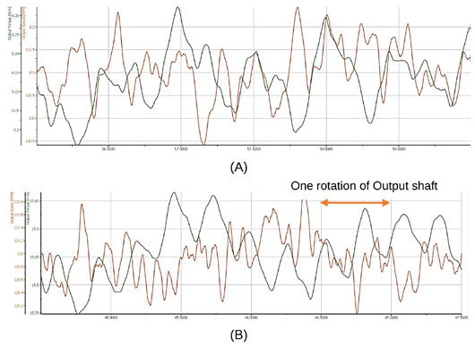
Figure 5 and Figure 7 show the torque and speed curves for healthy and damaged gearbox conditions. Each condition has 0 Nm and 15 Nm loads. Both torque and speed curves depict the steadiness of the power (proportional to the product of torque and speed) flowing through the system by generally showing opposite trends to each other. The variation in those curves over the period of three seconds confirms the randomness of the signal, hence categorizing it as a nonstationary signal. The FFT would assume the same signal as stationary, i.e., the signal not varying with time. This assumption ignores the local irregularity or fractals, and hence potentially any evidence of the fault existence. When the signal of one second period was FFT processed and plotted against the RMS amplitude in m/s2 (refer to Figures 6 and 8), the aforementioned cycloidal mesh frequencies can be observed.

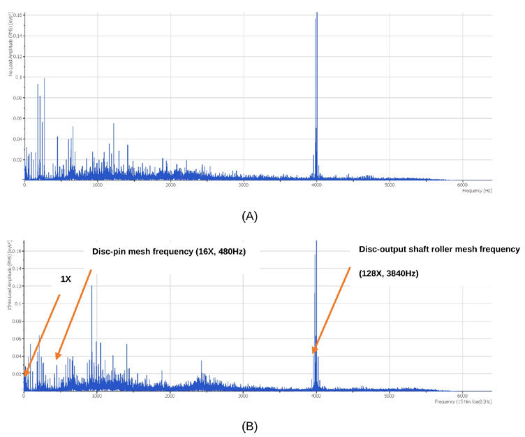
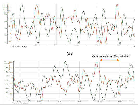
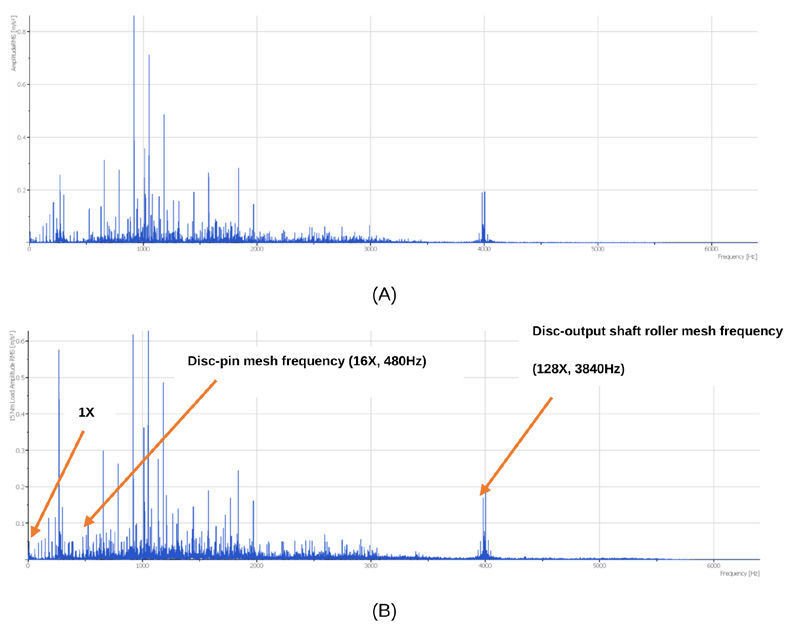
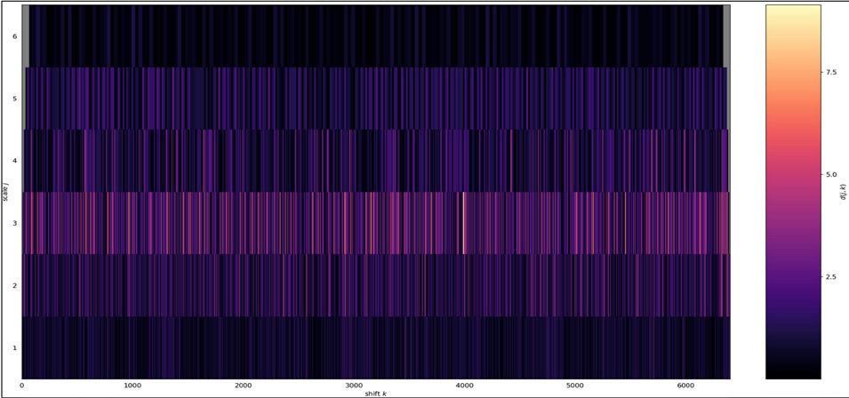
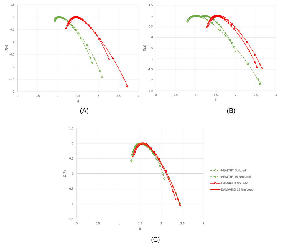
A typical way to diagnose any faulty machine using vibration is to compare its pre- and post-incident data, which means comparing the healthy (Figure 6) and the damaged reducer (Figure 8) graphs. However, apart from observing the higher amplitudes across the spectrum, it was incomprehensible to establish any relation with the fault by utilizing known frequencies (highlighted in graphs). Even at 16× order (disc-pin mesh frequency), where the fault was induced, no noticeable relative data change was observed. The same time period (one second) vibration data was then analyzed with WT, by plotting the Scalogram shown in Figure 9. As discussed in the “Introduction” section, the Scalogram or “Frequency vs Time” graph generally reveals the dominant frequencies at a time instant inside the non-stationary signal. Figure 9 shows a burst in localized activities, confirming the existence of mono- or multifractality in the signal generated by the damaged gearbox. Equations 4–8 were used to perform Multifractal analysis to extract wavelet coefficients that built the Scalogram, to derive the multifractal spectrum. The multifractal spectrum is plotted in Figure 10 for all three axes of vibrations: vertical, horizontal, and axial. The axis diagram, referred to in Figure 1, has the reducer shaft axis aligned with the vibration axial direction, and the remaining axes are in the radial direction of the cycloidal disc.

Each graph in Figure 10 consists of four curves showing different operating conditions of the gearbox: a healthy reducer with no load, a healthy reducer with 15 Nm load, a damaged reducer with no load, and a damaged reducer with 15 Nm load. Based on their positioning on the graph, the curves can visibly be sorted into healthy and damaged groups (green color and red color, respectively) in Figure 10(A) and Figure 10(B). The damaged gearbox’s curves are shifted towards the right side of the multifractal spectrum, making them separated from the healthy ones. It can be argued that the main cause of this distinction was the induced damage on the cycloidal disc. The worn-out surface on the disc generated singularities affecting the wavelet coefficients, subsequently creating a deviation in the multifractal spectrum in radial directions. The axial axis graph, Figure 10(C), does not show similar shifting, as the worn-out lobe of the disc would not have energy change in this direction. The loading conditions, 0 Nm and 15 Nm, do not noticeably influence the shifting in all three graphs.

Conclusion

The paper compares results of the two tests conducted on the same gearbox. The only difference between the two test setups was the condition of Cycloidal disc, depicting ‘healthy’ in one and ‘faulty’ in another. The multifractal spectrum clearly distinguished the vibration data with respect to their conditions, which Fast Fourier Transform graphs could not. This paper argues that the wavelet transform based multifractal analysis approach makes the Cycloidal gearbox diagnosis less ambiguous compared to FFT. This is mainly because the collected vibration signals were time dependent and the singularities in the signal cannot be captured using FFT. The multifractal spectra also showed that the load on the gearbox output shaft does not significantly influence the curve shifting or the Hölder coefficient. For the future work, it is worth exploring the ‘worn-out’ effect of other Cycloidal gearbox components, such ring gear pins, output rollers, on the multifractal spectrum and establish the changes to be utilized in fault diagnostics.

References

1. ANSI/AGMA 6002-D20, Design guide for vehicle spur and helical gears, 2020, AGMA.

2. R. B. Randall, Frequency analysis, 3rd ed. Naerum: Brüel & Kjaer, 1987.

3. K. G.-H. Svend Gade, “Technical Review: Non-stationary Signal Analysis using Wavelet Transform, Short-time Fourier Transform and Winger-Ville Distribution,” Bruel & Kjaer, 1996.

4. J. Morlet, G. Arens, E. Fourgeau, and D. Giard, “Wave propagation and sampling theory; Part II, Sampling theory and complex waves,” Geophysics, Vol. 47, No. 2, pp. 222–236, Feb. 1982, doi: 10.1190/1.1441329.

5. B. B. Mandelbrot, The Fractal Geometry of Nature. New York: W.H. Freeman and Company, 1977.

6. C. Meneveau and K. R. Sreenivasan, “Simple multifractal cascade model for fully developed turbulence,” Phys Rev Lett, Vol. 59, pp. 1424–1427, 1987.

7. D. Lin and R. Hughson, “Modeling Heart Rate Variability in Healthy Humans: A Turbulence Analogy,” Phys Rev Lett, Vol. 86, pp. 1650–1653, May 2001, doi: 10.17877/DE290R-16101.

8. H. Wendt, S. G. Roux, S. Jaffard, and P. Abry, “Wavelet leaders and bootstrap for multifractal analysis of images,” Signal Processing, Vol. 89, No. 6, pp. 1100–1114, 2009, [Online]. Available: http://dx.doi.org/10.1016/j.sigpro.2008.12.015

9. W. Du, J. Tao, Y. Li, and C. Liu, “Wavelet leaders multifractal features based fault diagnosis of rotating mechanism,” Mech Syst Signal Process, Vol. 43, No. 1, pp. 57–75, 2014, doi: https://doi.org/10.1016/j.ymssp.2013.09.003.

10. T. Figlus and M. Kozioł, “Application of the Multifractal Spectrum to the Analysis of Vibration Signals Generated During Testing of Selected Composite Materials,” Advances in Science and Technology Research Journal, Vol. 18, No. 7, pp. 123–137, 2024, doi: 10.12913/22998624/192616.

11. W. J. Staszewski and G. R. Tomlinson, “Application of the wavelet transform to fault detection in a spur gear,” Mech Syst Signal Process, Vol. 8, No. 3, pp. 289–307, May 1994, doi: 10.1006/mssp.1994.1022.

12. S. J. Loutridis, “Self-similarity in vibration time series: Application to gear fault diagnostics,” J Vib Acoust, Vol. 130, No. 3, 2008.

13. A. Puchalski and I. Komorska, “Data-driven monitoring of the gearbox using multifractal analysis and machine learning methods,” MATEC Web Conf., Vol. 252, 2019.

14. Komorska, K. Olejarczyk, A. Puchalski, M. Wiklo, and Z. Wolczyski, “Fault Diagnosing of Cycloidal Gear Reducer Using Statistical Features of Vibration Signal and Multifractal Spectra,” Sensors, Vol. 23, No. 3, 2023, doi: 10.3390/s23031645.

15. V. Cochran and T. Bobak, “A methodology for identifying defective cycloidal reduction components using vibration analysis and techniques,” in American Gear Manufacturers Association—American Gear Manufacturers Association Fall Technical Meeting 2008, San Antonio, TX, United States, 2008, pp. 8–32.

16. H. Wendt, “Contributions of Wavelet Leaders and Bootstrap to Multifractal Analysis: Images, Estimation Performance, Dependence Structure and Vanishing Moments. Confidence Intervals and Hypothesis Tests,” May 2008.

17. Sumitomo, “Cyclo Reducer Catalog,” 2025.